



A cloud-based miniscope for neurosurveillance of brain health and disease in freely behaving animals
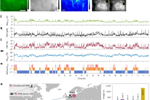
Main The ability to conduct continuous (≥24 h), neuroimaging of multiple physiological variables (for example neuronal activity (Neu ACT ), blood flow, blood volume, oxygenation and cellular dynamics) within the CNS microenvironment is crucial for characterizing preclinical models of CNS disease (Supplementary Table 1 ). We refer to this continuous multimodality neuroimaging capability as ‘neurosurveillance’ 1 . Neurosurveillance can empower us to elucidate the etiology, progression and therapeutic response of CNS diseases ranging from seizures to brain cancer, while simultaneously permitting their correlation with behavioral outcomes. Recent advances in miniaturized optical microscopes (‘miniscopes’ 2 ), have made neuroimaging in freely behaving, unrestrained animals a reality; however, most extant miniscopes are specifically designed to interrogate healthy brain function and acquire images with a single image contrast mechanism based on Neu ACT 2 or vascular function 3 , but usually not both, at a high frame rate (for example 10–20 Hz) over short durations (for example <2 h) (Supplementary Table 2 ). This short-duration, single-modality imaging approach limits the utility of most miniscopes for conducting neurosurveillance in preclinical models of CNS disease because many pathological changes occur over substantially longer timescales (for example >24 h to days), and often involve the dysregulation of both neuronal and vascular function. Moreover, technical hurdles such as the lack of an architecture for remote miniscope operation to enable continuous imaging for ≥24 h; cloud-based image streaming to enable operators to check image acquisition in real-time; photobleaching; image sensor overheating; a need for proprietary electronic and optical parts; and limited battery life, have made it challenging to conduct neurosurveillance of CNS disease models. To circumvent these limitations, we developed a miniscope system called the CloudScope, which integrates a three-dimensional (3D)-printed miniscope designed for long-term multicontrast neuroimaging with an internet of things (IoT) networked architecture. The CloudScope can track Neu ACT , cerebral blood flow (CBF), cerebral blood volume (CBV), intravascular oxygenation (Hb SAT ) and cells in vivo for neurosurveillance in freely behaving animals. CloudScope was implemented using inexpensive, commercially available, hobbyist or open-source components to encourage ubiquitous usage and enhancement by the broader neuroscientific community. Once the CloudScope has been mounted on an animal, its cloud-based architecture and image-acquisition scheme enable continuous multicontrast imaging for ≥24 h without sensor overheating or photobleaching, while permitting in vivo neuroimaging from anywhere in the world. We demonstrate the widespread potential of CloudScope via a host of continuous (≥24 h) neurosurveillance applications in healthy animals and CNS disease models that include: (1) predicting animal behavior from continuously acquired Neu ACT data with deep learning (DL); (2) characterizing neurovascular changes in the brains of freely behaving healthy mice; (3) assessing seizure-induced disruptions and subsequent recovery of Neu ACT and neurovascular function; and (4) an in vivo assay for cellular and vascular phenotyping during brain tumor evolution. We believe these innovations and their broad applicability make the CloudScope a powerful tool for characterizing long-term, in vivo changes in the CNS microenvironment in health and disease. Results CloudScope enabled remote neurosurveillance over 24 h in healthy freely behaving animals An IoT architecture (Fig. 1a ) permits CloudScopes connected to the internet via Wi-Fi, to be used individually (Fig. 1b ) or assembled into a ‘miniscope bank’, for example in an animal facility or a lab (Extended Data Fig. 1a–d and Supplementary Video 1 ). Users can log into a CloudScope server from anywhere in the world, set image acquisition parameters, initiate image acquisition and observe in vivo experiments in real-time via a graphical user interface (GUI; Extended Data Fig. 1e–g ). The CloudScope (Fig. 1c ) weighs <3.5 g and can be mounted on the head of a freely behaving mouse (Fig. 1d ) to acquire images over a wide field of view (FoV; ~3 × 3 mm 2 ), at a high spatial resolution (~5.5–7 μm; Extended Data Fig. 1h–q ). Supplementary Table 2 provides a comparison of the CloudScope with extant miniscopes. To ensure affordability and widespread adoption, CloudScope’s control circuitry was implemented using hobbyist electronics and off-the-shelf components. A flexible printed circuit board (PCB) (Fig. 1b,c , ‘flex PCB’) housed the electronics to control a 10-bit image sensor and allowed unimpeded head motion. A surface mount blue LED (wavelength range = ~453 ± 20 nm) and a green (GR) LED (wavelength range = ~530 ± 20 nm), a vertical cavity surface emitting laser diode (LS, center wavelength = 670 nm or 680 nm), an aspheric lens (focal length = 4.6 mm) and a long-pass filter (cutoff wavelength = 510 nm) enabled multicontrast imaging (pupil size = ~1.1 mm and magnification = ~×0.7) with green fluorescence (FL), intrinsic optical signals 4 (IOS) and laser speckle contrast 5 (LSC) (Fig. 1e ). Unlike in ref. 6 , additional PCBs for mounting LEDs were not required, as LEDs were directly soldered on to 32-gauge wires (diameter = ~200 μm; Fig. 1c ) and any strain on the solder joints relieved by affixing those wires to 3D-printed holes via cyanoacrylate glue. A 3D-printed slider (~2-mm sliding range; Fig. 1e ) and lock screw enabled convenient focusing (Supplementary Fig. 1 ). The 3D-printed head-mount enabled easy attachment of the CloudScope to the mouse’s head (Fig. 1d and Supplementary Fig. 2a–f , working distance of ~2 mm). A meter-long flat flexible cable (FFC; ~200-μm thickness) connected the CloudScope to a control module mounted on the cage (Fig. 1b ), which permitted the animal to move freely during 24-h imaging sessions (Supplementary Videos 2 and 3 ). The control module handled communication to/from the cloud-server (Fig. 1b and Supplementary Fig. 3 ). Within it, a Raspberry Pi and a Teensyduino were configured in an ‘initiator–responder’ arrangement to manage image acquisition, Wi-Fi-based image transfer, and illumination control. Acquired images were saved to a USB drive (~64 GB to 1 TB) connected to the Raspberry Pi and analyzed offline. Fig. 1: CloudScope enabled remote neurosurveillance over 24 h in healthy freely behaving animals. a , Schematic illustrating the cloud-based IoT architecture that supports internet access to multiple CloudScopes. CloudScopes can be housed in a laboratory or an animal facility and connect to a cloud-based server via local Wi-Fi. b , Schematic of the system setup. A control unit placed above the cage handled all communications with the cloud-based server. A USB attached to the control unit enabled local image storage. The control unit was linked to the CloudScope via a 1 m FFC, a flex PCB integrated with a 30-cm ribbon cable, for power and image transfer. An additional set of thin 32 G (200-μm diameter) wires carried power from the control unit to the CloudScope’s illumination sources. c , A photograph of the CloudScope, showing the 30-cm ribbon cable and integrated flex PCB, and 32 G wires. d , Photograph of the CloudScope mounted on a freely behaving mouse. e , Schematic illustrating key optical components of the CloudScope. Blue and green LEDs (453/530 ± 20 nm), a laser diode (670 nm or 680 nm), a fixed focus lens (lens, f = 4.6 mm) and a long-pass filter (cutoff of 510 nm) for imaging green FL, IOS and LSC over the same cortical FoV. Image focus was achieved by manually adjusting the linear focusing slider, which was then locked in place with set screws. f – h , Maps of neuronal calcium dynamics (via FL of GCaMP6s-bound Ca 2+ in neuropil or neuronal soma) ( f ); microvascular architecture (via IOS) ( g ); and CBF (via LSC) ( h ) from a 3 × 3 mm 2 FoV in the mouse cortex (center = −2/+2 mm AP/ML with respect to the bregma) simultaneously acquired with the CloudScope. i , Animal behavior was captured via a separate behavioral camera that was synchronized with multicontrast neuroimaging. j – n , A 24-h time-series of Neu ACT ( j ); CBV ( k ); CBF ( l ); intravascular Hb SAT ( m ); and the animal’s behavioral state ( n ) recorded from a freely behaving mouse. Neuroimaging time-series shown are spatial averages from the parenchyma (excluding surface vessels) and denoised with a 30-s median filter for visualization purposes. The behavior of the animal was classified as belonging to one of three Behavior SYL (MM, INT or R). The light–dark cycle is denoted by gray–black time axis labels. o , A world map illustrating the locations from which the CloudScope was remotely accessed. These remote access points included UK (London), China (Ningbo), Sri Lanka (Colombo), Australia (Sydney), South Africa (Pretoria) and Brazil (Brasilia). Users from these locations are labeled as User 1..., User 6, respectively, with pseudocolored traces indicating CloudScope access. Inset on the top-right shows the number of images acquired by each user (note, users acquired images of a test pattern to ensure compliance with experimentation rules in the participating countries). As highlighted by the inset on the top-left, users gained access to the CloudScope housed in Baltimore, MD via an Amazon Web Services (AWS) server located in Ashburn, VA. Panel b created in BioRender; Thakor, N. https://biorender.com/7828ikd (2026). The schematic in e was created with SolidWorks 2021 (Dassault Systèmes). The world map in o was created using the Python package ‘Plotly’. Scale bar, 500 μm ( f ). H, high; L, low. The head-mounted CloudScope (Fig. 1d ) permitted assessment of multiple neurophysiologic variables, including (1) changes in Neu ACT via GCaMP6s-bound Ca 2+ in neuropil and neuronal soma 7 (Fig. 1f and Supplementary Fig. 4 ) or tracking of fluorescent dyes and cells via the FL channel; (2) mapping changes in CBV (∆CBV, with total hemoglobin content or ∆HbT; Fig. 1g ), oxy-/deoxy-hemoglobin content (∆HbO and ∆Hb) and intravascular oxygen saturation (Hb SAT ) via the IOS channels; (3i) and quantifying changes in CBF (∆CBF) via the LSC channel (Fig. 1h ). Users could operate the CloudScope in ‘livestream’ mode to fine tune image acquisition parameters for each contrast mechanism (Supplementary Table 3 ) or conduct high-speed (up to ~19 fps; Extended Data Fig. 2 ) imaging using a single contrast mechanism. Examples include discriminating cerebral arterioles from venules by tracking the transit of an intravenously injected FL tracer (size 512 × 512 pixels, resolution = 7 μm, speed = ~9 fps; Supplementary Video 4 ) or visualizing microscopic-scale functional connectivity patterns with high temporal resolution image acquisitions (size 128 × 128 pixels, resolution = ~25 μm, speed = ~19 fps; Extended Data Fig. 2 and Supplementary Video 5 ). Users could then switch to a ‘sequential stream’ mode to automatically cycle through each channel for a predefined period (for example every ~5 s) while minimizing overheating of the image sensor (Supplementary Fig. 5 ). Cyclically acquired images were resampled at fixed time steps to correct for minor variations in frame rate and obtain concurrent multicontrast datasets. CloudScope operation (for example for >10 min of live streaming or >24 h of sequential streaming; Supplementary Videos 6 and 7 ) did not result in excessive heating or photobleaching (Supplementary Figs. 6 and 7 ). Animal activity was captured via a separate ‘behavioral camera’ (Fig. 1i ), and annotated offline into three ‘behavioral syllables’ 8 (Behavior SYL ): minimally mobile (MM), intermediate (INT) or running (R) (Fig. 1n ). These technical advances permitted us to continuously correlate Neu ACT , CBV, CBF and Hb SAT changes with animal behavior over >24 h (Fig. 1j–n ). As expected 9 , epochs of increased animal activity were accompanied by elevated Neu ACT and CBF, vasodilation (increased CBV), increased HbO, decreased Hb, and increased Hb SAT (for example epochs E1, E2, E3 and E4; Extended Data Fig. 3 ). In some instances, elevated CBF, CBV and Hb SAT , which may be linked to the hemodynamic correlates of sleep or arousal 10 , were observed without proportionate changes in Neu ACT or behavior (for example epoch E4*; Extended Data Fig. 3 ). Conversely, we observed a suppression of Neu ACT concurrent with an increase in Hb SAT under isoflurane anesthesia (in n = 5 mice) that was consistent with prior reports of decreased electroencephalogram (EEG) activity and reduced cerebral metabolic rate of oxygen induced by that anesthetic 11 (Extended Data Fig. 4 ). Collectively, long-term neurosurveillance via multicontrast imaging as well as the CloudScope’s remote access capabilities (Fig. 1o ) create a platform for interrogating the complex interplay between Neu ACT and vascular dynamics in freely behaving animals. Deep learning can predict individual animal behavior from 24-h neurosurveillance data DL is fast gaining popularity as an approach for predicting animal behavior from neuroimaging data 12 . While non-DL methods such as complex-PCA 13 , dynamic functional connectivity (dFC) 14 or co-activation patterns (CAPs) 15 , can be used for behavioral classification, tradeoffs between their specificity versus sensitivity, or the need to identify a reference region often precludes their use for predicting animal behaviors (for example MM, INT or R) from short-duration (for example 1 min) and limited FoV (only 3 × 3 mm 2 ) neurosurveillance data. Conversely, the limited amount of neuroimaging data available per animal from benchtop-based neuroimaging systems (for example <2 h) often necessitates pooling data from multiple animals 12 , making it unfeasible to account for characteristics unique to individual animals. To address this, we hypothesized that we could use neurosurveillance-based data for optimizing a DL model pretrained on nonbiological inputs to predict ‘individual animal’ behavior from its own neuroimages (Fig. 2a and Supplementary Fig. 8a–e ). Fig. 2: Deep learning can predict individual animal behavior from 24-h neurosurveillance data. a , Distributions of Neu ACT (μ Neu ACT ) corresponding to MM, INT and R Behavior SYL over 24 h. Data shown are from M2. b , Schematic illustrating the DL pipeline. First, 1-min intervals, during which, an animal consistently maintained a Behavior SYL (MM, INT or R) were identified and the corresponding Neu ACT images grouped together to create 1-min ‘Neu ACT blocks’. Key components of the pipeline such as the pre-processing steps, the ResNet50 unit, the BiLSTM unit and the FC layer are also shown. Additionally, the class scores created at the end of the DL pipeline were input into a gradient class activation mapping (Grad-CAM) unit to identify the spatial location of fea
Source: Nature